50 Hz · Europe's electricity, live

Building a simulation based on real numbers is a small challenge I had wanted to take on for a long time. I had already tried it with Paradise, where I simulated life in an underground city: the oxygen, water, calories and electricity its inhabitants need every day, everything the city spends to keep going.

With 50 Hz, I wanted to go a bit further on the subject of energy, and step out of the closed city to look at the real one. How electricity is produced in Europe, by which means, how it's stored and given back, and how it moves from one country to another. That's why I built 50 Hz.

The name comes from a quirk of electricity: it can barely be stored. Every second, Europe has to produce exactly what it consumes, and the sign that the balance holds is the frequency of the current, which stays stuck at 50 Hz. Everyone uses it, and almost nobody knows where the power coming out of their socket comes from.

What it is

50 Hz is a map of Europe that shows where electricity is produced, where it's consumed and what countries trade with each other, live. It's online at 50hz.kevin-dev.com.

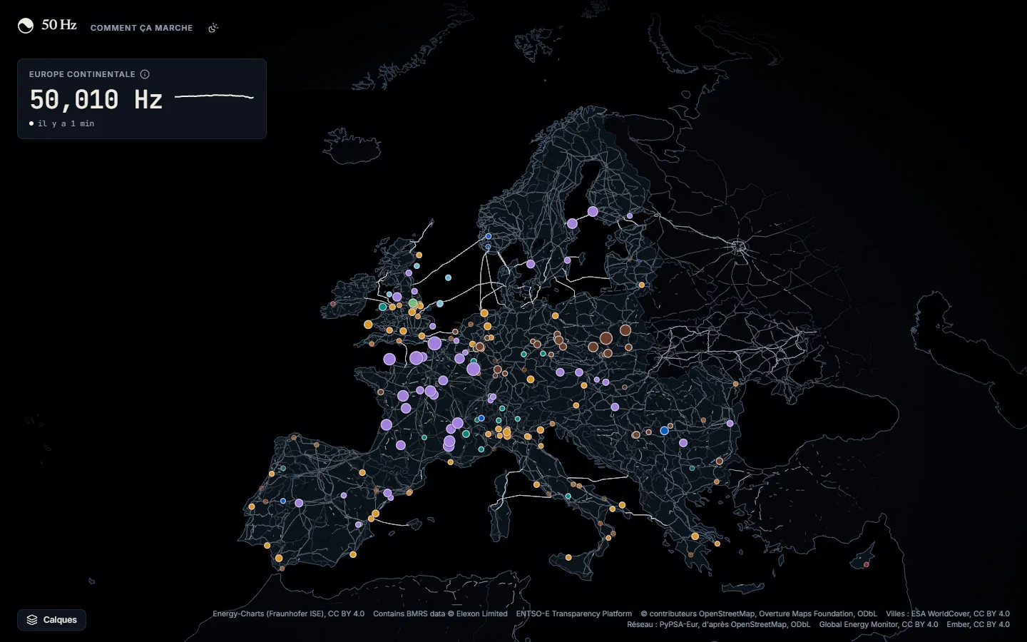
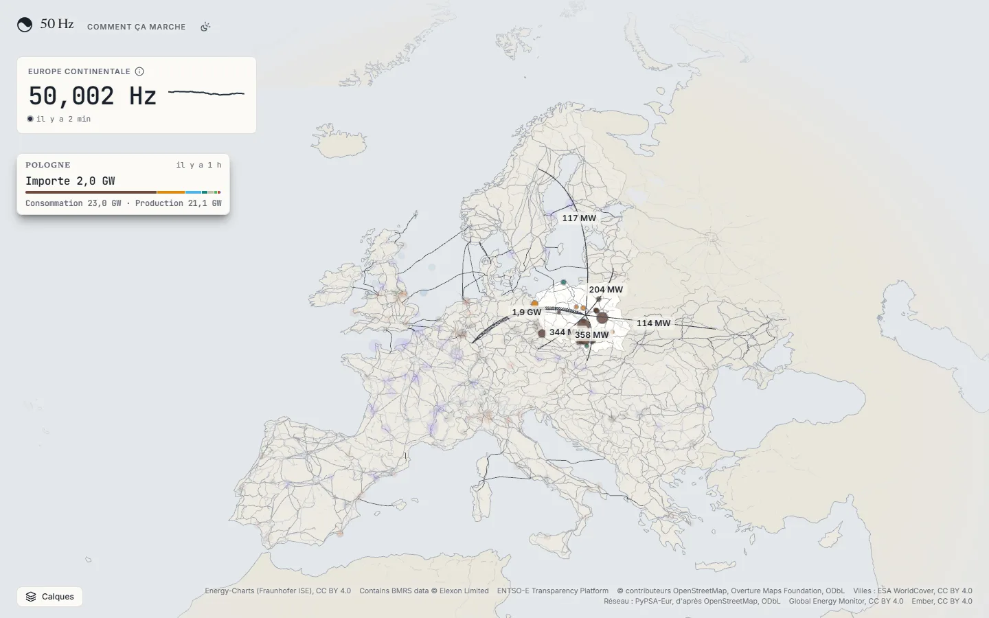
Top left, there's the frequency of the continental grid, measured every second.

On the map, you see the high-voltage grid and a disc for each large power plant. Its colour gives its type, and its size follows its capacity.

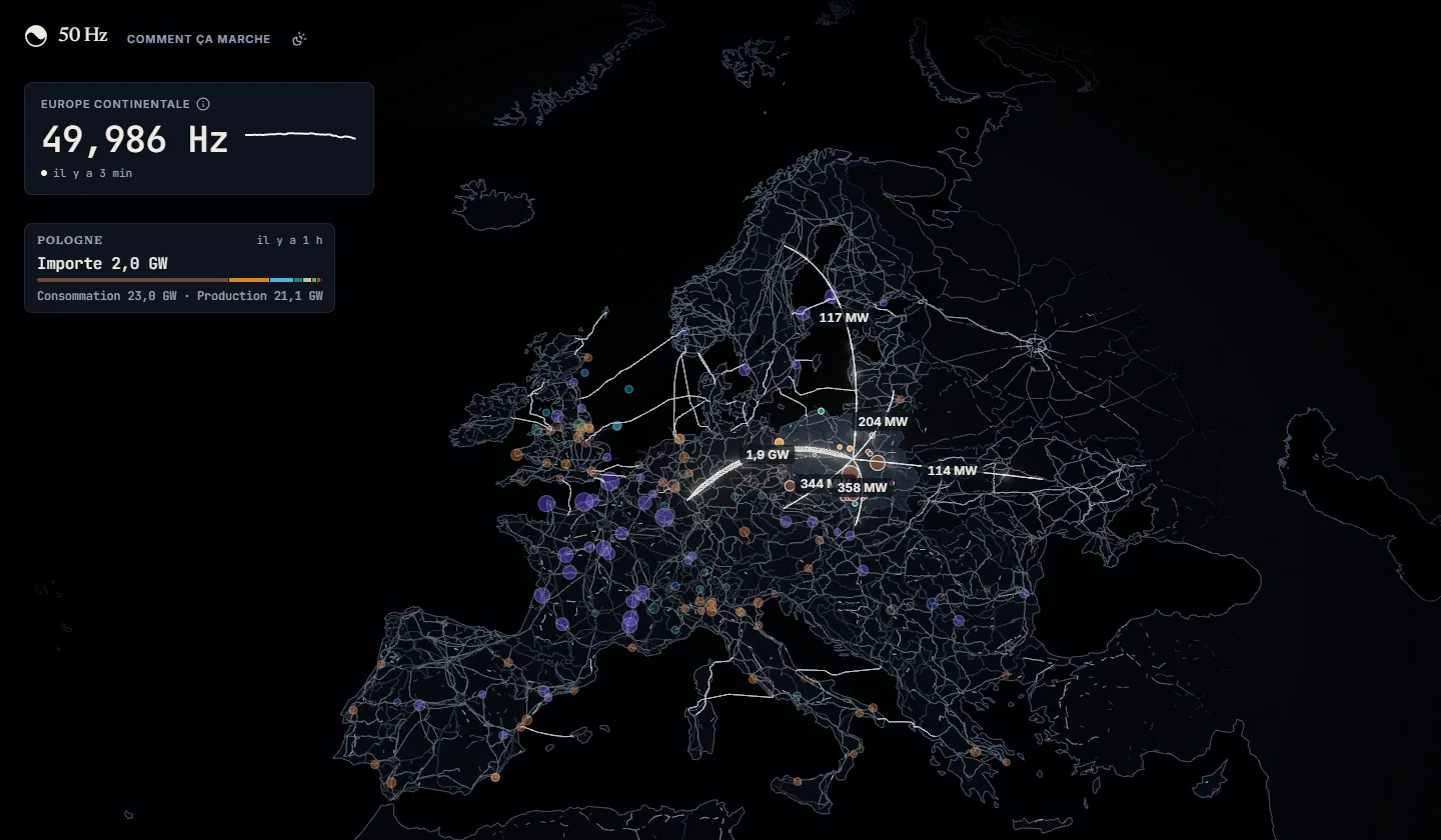
When you hover a country, its smaller plants show up and its exchanges with its neighbours are drawn as arcs. A card in the corner gives what it produces, what it consumes, and whether it imports or exports.

Clicking a plant opens its sheet: its capacity, its rank in the country, its share of its type, and what that type is producing in the country right now. Below that, a model of the site.

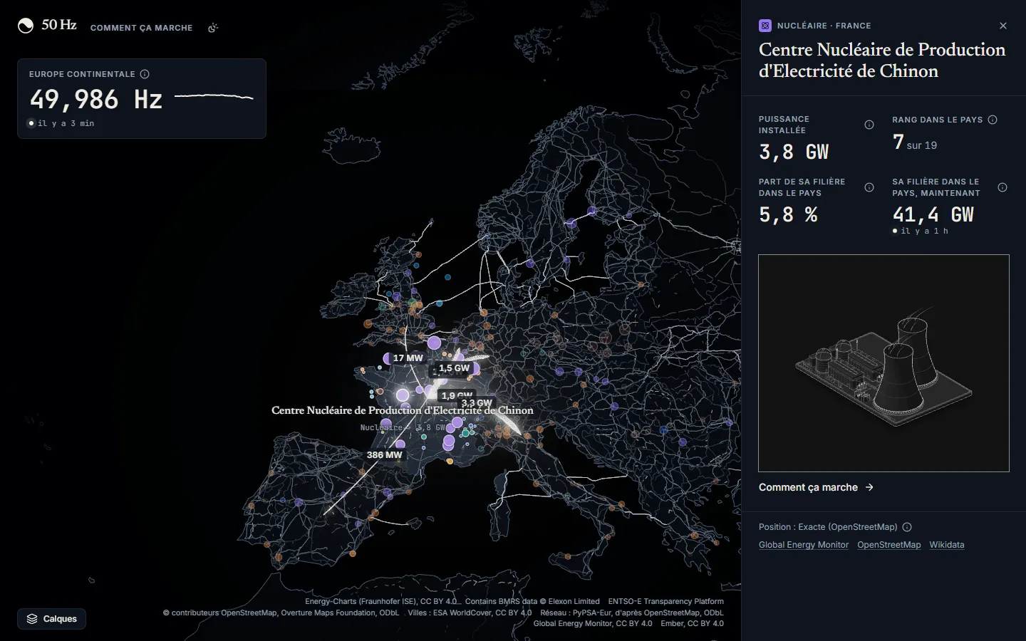
That model leads to the second half of the site, "How it works".

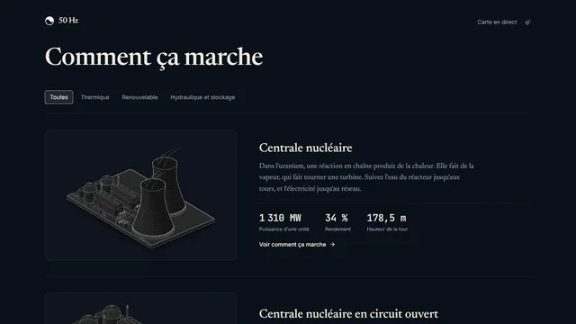
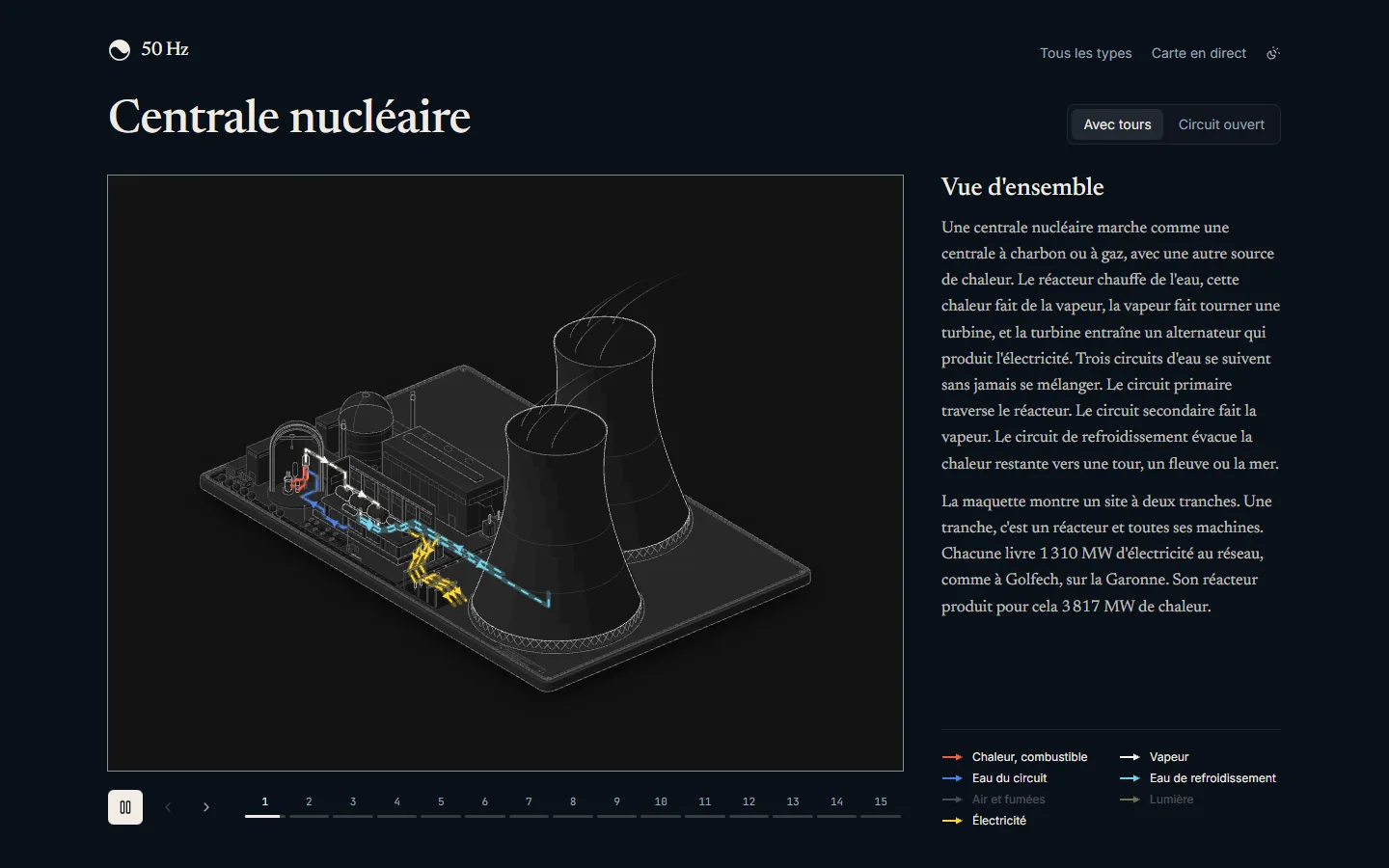
It covers each kind of plant: nuclear, dam, offshore wind, combined cycle gas, batteries… Each one has its large figure, with numbered steps at the bottom that you go through with the arrows.

Nuclear has fifteen, from fission to the substation. The water circuits, steam and electricity are in colour, so you can follow them from one step to the next.

The data

Everything on the map comes from public sources, credited at the bottom of the screen.

What you see	Where it comes from
Generation, load and exchanges of continental Europe	ENTSO-E Transparency Platform, with access to request
Generation, load and exchanges of Great Britain	Elexon BMRS, open to everyone
Continental frequency, every second	Energy-Charts by Fraunhofer ISE
Power plants, their capacity and location	Global Energy Monitor matched with OpenStreetMap
The high-voltage grid	PyPSA-Eur, based on OpenStreetMap
Installed capacity of each country	Ember

All this data is public. But each country publishes it at its own pace: some every fifteen minutes, others every half hour or every hour, and not all with the same delay.

The plants come from two databases that are each wrong in their own way: Global Energy Monitor often has the right capacity but a rough location, OpenStreetMap has the right location but not always the capacity. A Python script matches them, first by their shared identifiers, then by distance, and a file of sourced corrections catches the cases the algorithm misses. In the end, the map shows almost 14,000 plants of 10 MW and more.

Each country's sources

For each country, we need to know where its generation, its load and its exchanges with each neighbour come from. All of it lives in a single file, the source sheet, with one rule: a single source per number, the best one available. The rest of the code has no condition or switch on sources, it reads the sheet.

It starts by saying which provider can read which measure:

type MeasureProviders = {
  generation: 'entsoe' | 'elexon'
  load: 'entsoe' | 'elexon'
  exchange: 'entsoe' | 'elexon'
  frequency: 'elexon' | 'energy-charts'
}

export type ProviderOf<M extends Measure> = MeasureProviders[M]

Then it holds three tables. The first gives, for each area of the map, the countries it covers and the source of its generation and load:

export const AREA_SOURCES = {
  'DE-LU': { countries: ['DE', 'LU'], zones: ['DE-LU'], generation: 'entsoe', load: 'entsoe' },
  'FR': { countries: ['FR'], zones: ['FR'], generation: 'entsoe', load: 'entsoe' },
  'GB': { countries: ['GB'], zones: ['GB'], generation: 'elexon', load: 'elexon' },
  'IE-SEM': { countries: ['IE', 'GB-NIR'], zones: ['IE-SEM'], generation: 'entsoe', load: null },
  // …
}

An area can cover several countries: Germany and Luxembourg share the same electricity market, and ENTSO-E publishes them together. A null says plainly that no source publishes the number, like the load of Ireland.

The second table lists each border with its source, one line per pair of neighbours:

export const BORDER_SOURCES: [BiddingZone, BiddingZone, ProviderOf<'exchange'>][] = [
  ['BE', 'FR', 'entsoe'],
  ['DE-LU', 'FR', 'entsoe'],
  ['GB', 'FR', 'elexon'],
  // …
]

The third gives the frequency of each grid: Energy-Charts for the continent, Elexon for Great Britain, and nothing for the Nordic countries and Ireland, which nobody publishes live.

To choose a source, I look at what it really measures. ENTSO-E covers the whole continent with the same definitions. For Great Britain, Elexon gives its six interconnectors cable by cable. And for exchanges, I only take physical flows, what actually goes through the cables, not the commercial schedules that RTE publishes in éCO2mix, for example.

Everything is typed from this sheet. Writing frequency: 'entsoe' doesn't compile, since ENTSO-E doesn't publish the frequency. The registry that fetches the data has the same shape:

const FETCHERS: { [M in Measure]: Record<ProviderOf<M>, MeasureFetcher<M>> } = {
  generation: { entsoe: entsoeGeneration, elexon: elexonGeneration },
  load: { entsoe: entsoeLoad, elexon: elexonLoad },
  exchange: { entsoe: entsoeExchange, elexon: elexonExchange },
  frequency: { 'elexon': elexonFrequency, 'energy-charts': energyChartsFrequency },
}

It must have a reader for every provider the sheet allows, and no other. Tests check the rest: no area or border is declared twice, every border links two countries of the map, and Elexon only serves Great Britain. Changing source means changing one value in the sheet.

Never show a fake number

The other rule is to invent nothing. I had already set it for myself on Paradise, where every number in the city came from a real source. Here, it's written down in the project's decisions, so every Claude session finds it. The frequency of the Nordic countries and Ireland isn't published live anywhere, so the dial doesn't show it.

But there's another, quieter trap. A country is a dozen series: each type of generation, the load, each border. They don't all arrive at the same time, and adding the 2 pm solar to the 1 pm nuclear would give a total that never existed. So a country shows at the latest instant all its series cover:

export function latestCompleteInstant(series: PowerReading[][]) {
  const candidates = [...new Set(series.flat().map((reading) => reading.time.getTime()))].toSorted(
    (first, second) => second - first
  )

  for (const instantMs of candidates) {
    const readings = readingsAt(series, instantMs)

    if (readings) {
      return { time: new Date(instantMs), readings }
    }
  }

  return null
}

We start from the most recent instant and go back to the first one where nothing is missing. If that moment is two hours old, so be it: the map still shows it, with "2 h ago". I preferred that to an empty country, because a visitor who lands on the page and sees gaps everywhere will wonder whether the site works.

Official sources get things wrong too. On 2 November at noon, ENTSO-E published 7,707 MW of solar for Moldova, which has only a little over 700 MW of panels installed according to Ember. Since then, each value is compared with twice the country's installed capacity, and anything above is dropped, as if nothing had been published. The margin is wide on purpose: the ceiling should only catch errors of an order of magnitude, not a real record day.

What happens behind the scenes

The app uses the same stack as this site: AdonisJS with Inertia and React 19, Postgres, all in Docker containers on my VPS, under Dokploy. Next to the web server runs a second container, the worker, which polls each source at its own pace (every 15 minutes for ENTSO-E, much more often for the frequency) and stores the numbers as they arrive.

Everything that doesn't change live is prepared ahead of time by a Python pipeline, run with uv: the basemap, the high-voltage grid, the towns of the night background, the power plants. Each product has its own command, which projects, simplifies and writes compact binary files, committed into the app. Regenerating them on every build would have taken nine minutes and more than two gigabytes of sources for the basemap alone.

The map itself is drawn with three.js and React Three Fiber, without any mapping library. The research recommended MapLibre and deck.gl, with a gigabyte and a half of tiles. I preferred plain three.js: we need no globe, no choice of projections and no map styles, just a flat Europe where we control every pixel. Coordinates are projected once and for all in the pipeline, in the European Union's official equal-area projection (EPSG:3035), and the browser only has to display them. The plants are a single point cloud, with a shader that decides on every frame which ones to show depending on the zoom: 1 GW and more over Europe, around 300 MW over a country, all of them up close.

Three days and quite a few turns

The project started on 1 November and has been online since the evening of the 3rd. That sounds fast, but it changed direction several times along the way.

3D models, then none at all

In my head, at first, each plant was going to have its own 3D model, placed at its real coordinates. I installed Blender on my PC, and Claude drove it through Python scripts, without ever opening the interface: one script per kind of plant, exported for the web, with several levels of detail. Here's what it looked like for a nuclear plant:

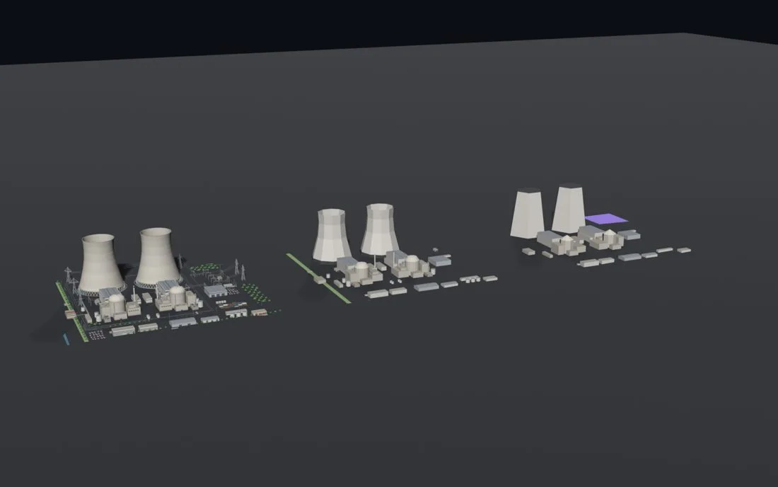
I found them too simple, so we redid all of them, with more detail and about ten agents in parallel. But once on the map, the problem was elsewhere. Each site had a ground coloured by its type, and between the names of every country, the glowing arcs and those rectangles on an empty background, the map had become hard to read. Patches of green, orange or purple grass right in the middle of Germany.

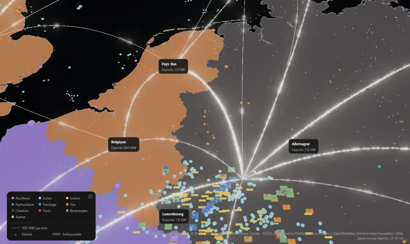
Meanwhile, I had come across the Anatomy skill, which draws very detailed isometric figures of a machine, in SVG. We were using it for the plant sheets, and the figures were nicer and clearer than the 3D models. I figured we didn't need both. We kept the figures, redrawn as whole sites at real scale (one unit, one metre), and removed all the 3D: the Blender project, the sixteen models, their loading on the client, nearly 25,000 lines. On the map, a plant went back to being a simple disc, like on the reference maps.

A map you want to look at

To replace the empty black background, I studied the maps that already exist on the subject. On Open Infrastructure Map, I really like seeing every line, every pylon, every substation, and the towns around them. You can really see the path the power takes. I didn't want a copy, but that level of detail, mixed with our exchanges between countries, seemed interesting.

So we added the high-voltage grid, from 220 to 750 kV, with its substations, and a discreet night scenery: towns, water, main roads. The 20 kV lines and the buildings were left aside, because they would have required a tiling system. Later, I also asked for a light version of the site, map included, and for the neighbouring land to fade into the sea instead of stopping dead at the edge of the screen.

Working with Claude

All the code of 50 Hz was written by Claude Code, but not in a single conversation. A main conversation supervised the project for the three days, and it started other conversations for each piece of the work. It's a recent Claude Code feature: sessions that start and talk to each other.

Questions first

I now start all my projects with a round of questions and answers. I use the grill-me skill by Matt Pocock for it, which I adapted: Claude asks every question to settle, one by one, with a recommendation for each. Which countries to cover, what capacity threshold for the plants, what to do with a country that publishes nothing, which licence for the plant database… That's where I ruled out MapLibre.

It forces me to question what I really wanted to cover, and to put down in black and white what I want before the first line of code.

With those answers, we wrote the specification in a Claude document. It's a shared document that I can edit myself, and it was used to follow the whole project: the vision, the rules, the sources, the decisions and what was still open.

A supervisor and sessions

After that, the main conversation became the supervisor. It kept the big picture and handed out the tasks. For each piece (the basemap, ingestion, the figures, the design), it wrote a full brief and suggested a new session, which I approved with one click. Each session had a single responsibility and its own branch, and several ran at the same time. When one of them was done or stuck, it wrote to the supervisor, which gave me the summary.

When I wasn't available, I started the long, heavy tasks, like generating the 3D models or exporting the night background. They ran without me needing to watch what was going on.

My rules

In the projects I build with Claude, I start by setting the rules I like to work with. For 50 Hz:

• one module per domain, and each module is only imported through its public entry point;
• no useless comments, naming carries the intent;
• function and file names that say what they do, and booleans prefixed with is or has;
• Tailwind classes directly in the components, not in constants;
• one commit per feature, rather than a string of small commits;
• the app isn't in production, so no migrations or compatibility for data that doesn't exist.

As on this site, the ones that can be checked became lint rules. And before each merge, the session that did the work had to review everything it produced and give me a report: what's fixed, what's left and why, what's waiting for my decision.

ADRs

Every important choice is written down in an ADR, a short document that says what we decided, why, and what we ruled out. It describes the decision in force: it's rewritten when the decision changes, and the history stays in git.

Thanks to them, a new Claude session knows every choice already made before touching the code, and doesn't retry an abandoned idea. And it's documentation that's just as useful to a developer like me as to an agent.

What's still mine

Claude wrote all the code, did the research, drew the figures and wrote the texts. My role was to lead. I decided which tasks to tackle and in what order, and I gave my ideas on how to approach certain subjects: three.js rather than MapLibre, one source per number, no fake numbers, dropping the 3D.

Every time a session finished, I skimmed the code to spot ways of doing things I didn't like. And when Claude summarised what was left to do, I took the time to understand what it was saying, and to rephrase it with it. That's how I stayed in the project from start to finish, and kept it moving. It's also how I spotted inconsistent organisation choices that would have made the code hard to follow in the end. The source sheet came from that: I couldn't keep track of the sources anymore, and it was the sign that the logic was badly organised.

Where the project stands

50 Hz has been online since 3 November. For now, it's mostly a live map: the simulation part, which got me started on the project, is still to come. It's planned for later, with the option to cut a power plant to see the frequency react, and to replay the Iberian blackout of 28 April 2025. Before that, there's the map on mobile, and a view that follows the power all the way to your home, from the nearest substation. The code stays private for now.